Introduction to Pandas

The basics

Pandas is a Python library that provides data structures and data analysis tools. Pandas is often used in data science, machine learning, and NLP. It allows us to work with data in a way that is similar to a spreadsheet. Essentially, we can perform all the operations that we’ve done in previous Notebook but on a larger scale, dealing with large amounts of data/text.

Pandas also allows us to easily import data from various file formats such as CSV, Excel, SQL, and JSON. We can also export data to these formats.

Usually, we would work with a data that comes from a file stored on your computer, like an Excel spreadsheet, a CSV file or (god forbid) a SPSS file. But since we are working in Colab, we will import data from a file I stored on GitHub.

It’s a text dataset which should feel somehwat familiar - it stores textual information from the Lord of the Rings movie scripts. Before we start working with the data, let’s load the Pandas library.

In Python, loading software libraries is called importing. Majority of libraries are imported into Python as objects which have their own methods and attributes.

If you recall the previous notebook, we call methods and attributes of objects by using the dot operator. For example, if we have a library called pandas, we can call its methods by using the dot operator like this: pandas.method_name(). To avoid always typing the full name of the library, we usually import it with an alias. The alias is a shorter name that we can use to call the library’s methods.

This is why you will often see the following import statement in Python code:

import pandas as pd

Here pd is the alias for the pandas library.

First Pandas method we will use is the read_csv() method. This method reads a CSV file and returns a DataFrame object. A DataFrame is a two-dimensional data structure that looks like a table. It has rows and columns, and each column can have a different data type. We’ll see it in action in the next cell.

I’ve assigned the URL of the dataset to the url variable. We will use this variable to load the dataset and store it in the data variable.

url = 'https://gist.githubusercontent.com/atomashevic/9be5289d13fc430e4a8096ef3cddd5f7/raw/8d9bd9d6cfd3b1e4d102880457976db2ec032039/lotr.csv'

data = pd.read_csv(url )

Data Frames

Let’s examine the structure of the LOTR data frame. We can just type in the variable name and Colab will offer a nice spreadhseet-like view of the data.

data

	char	dialog	movie
0	DEAGOL	Oh Smeagol Ive got one! , Ive got a fish Smeag...	The Return of the King
1	SMEAGOL	Pull it in! Go on, go on, go on, pull it in!	The Return of the King
2	DEAGOL	Arrghh!	The Return of the King
3	SMEAGOL	Deagol!	The Return of the King
4	SMEAGOL	Deagol!	The Return of the King
...	...	...	...
2382	PIPPIN	Merry!	The Return of the King
2383	ARAGORN	Merry!	The Return of the King
2384	MERRY	He's always followed me everywhere I went sinc...	The Return of the King
2385	ARAGORN	One thing I've learnt about Hobbits: They are ...	The Return of the King
2386	MERRY	Foolhardy maybe. He's a Took!	The Return of the King

2387 rows × 3 columns

There are several things to unpack here. The first thing we see is that the table has three columns: char, dialogue, and movie. Each row represents a character’s dialogue from one of the three Lord of the Rings movies. The char column contains the name of the character who speaks the dialogue, the dialogue column contains the actual text of the dialogue, and the movie column contains the name of the movie the dialogue is from.

At the end we see that we have 2390 rows in total. This means that the dataset contains 2390 dialogue lines from the three Lord of the Rings movies.

I’ve said that dataframes are complex data structures. This means that within this data object we can access different parts of the data. For example, we can access the char column by typing data['char']. This will return a Pandas series object which is a one-dimensional data structure that looks like a list.

Give it a try in the next cell.

# Print the names of all characters
data['char']

0        DEAGOL
1       SMEAGOL
2        DEAGOL
3       SMEAGOL
4       SMEAGOL
         ...   
2382     PIPPIN
2383    ARAGORN
2384      MERRY
2385    ARAGORN
2386      MERRY
Name: char, Length: 2387, dtype: object

The second notable thing about pandas data frames is that every data frame object has built-in methods that allow us to perform various operations on the data. For example, we can use the head() method to display the first five rows of the data frame. This is useful when we want to quickly check the structure of the data set we are seeing for the first time.

data.head()

	char	dialog	movie
0	DEAGOL	Oh Smeagol Ive got one! , Ive got a fish Smeag...	The Return of the King
1	SMEAGOL	Pull it in! Go on, go on, go on, pull it in!	The Return of the King
2	DEAGOL	Arrghh!	The Return of the King
3	SMEAGOL	Deagol!	The Return of the King
4	SMEAGOL	Deagol!	The Return of the King

Exercise 1

Looking to the previous example with movie characters, a neat thing here would be too see how many unique characters are in the dataset.

We did something similar in the previous Notebook. Revisit that example and try to do the same here.

# Print the names of all characters, no duplicates

Now, can you retrieve the number of unique characters in the dataset?

# Retrieve the number of unique characters in the dataset

Pandas offers a more convenient way to do this. The unique() method returns an array of unique values in the column.

data['char'].unique()

array(['DEAGOL', 'SMEAGOL', '(GOLLUM', 'FRODO', 'MERRY', 'GIMLI',
       'GOLLUM', 'SAM', 'GANDALF', 'ARAGORN', 'PIPPIN', 'HOBBIT', 'ROSIE',
       'BILBO', 'TREEBEARD', 'SARUMAN', 'THEODEN', 'GALADRIL', 'ELROND',
       'GRIMA', 'FRODO VOICE OVER', 'WITCH KING', 'EOWYN', 'FARAMIR',
       'ORC', '\xa0GANDALF', 'SOLDIERS ON GATE', 'GOTHMOG', 'GENERAL',
       'CAPTAIN', 'SOLDIER', 'MOUTH OF SAURON', 'EOMER', 'ARMY', 'BOSON',
       'MERCENARY', 'EOWYN/MERRY', 'DENETHOR', 'ROHIRRIM',
       'GALADRIEL VOICEOVER', 'LEGOLAS', 'GALADRIEL', 'KING OF THE DEAD',
       'GRIMBOLD', 'IROLAS', 'ORCS', 'GAMLING', 'MADRIL', 'DAMROD',
       'SOLDIERS', 'SOLDIERS IN MINAS TIRITH', 'GANDALF VOICEOVER',
       'SOLDIER 1', 'SOLDIER 2', 'WOMAN', 'HALDIR', 'SAM VOICEOVER',
       'OLD MAN', 'BOROMIR', 'CROWD', 'ARWEN', 'ELROND VOICEOVER',
       'ARWEN VOICEOVER', 'ARAGORN ', 'HAMA', 'SHARKU', 'PEOPLE', 'LADY',
       'FREDA', 'MORWEN', 'EYE OF SAURON', 'ROHAN STABLEMAN', 'GORBAG',
       'ARGORN', 'GANDALF VOICE OVER', 'BOROMIR ', 'UGLUK', 'SHAGRAT',
       'SARUMAN VOICE OVER', 'SARUMAN VOICE OVER ', 'FRODO ', 'URUK-HAI',
       'SNAGA', 'GRISHNAKH', 'MERRY and PIPPIN', 'WILDMAN', 'STRIDER',
       'GALADRIEL VOICE-OVER', 'EOTHAIN', 'ROHAN HORSEMAN',
       'SAURON VOICE', 'SAM ', 'FRODO VOICE', 'GALADRIEL VOICE OVER',
       'FARMER MAGGOT', 'WHITE WIZARD', 'MERRY AND PIPPIN', 'GAFFER',
       'NOAKES', 'SANDYMAN', 'FIGWIT', 'GENERAL SHOUT', 'GRISHNAK',
       'URUK HAI', 'SARUMAN VOICEOVER', 'MRS BRACEGIRDLE',
       'BILBO VOICEOVER', 'PROUDFOOT HOBBIT', 'GATEKEEPER', 'GATEKEEPR',
       'MAN', 'CHILDREN HOBBITS', 'BARLIMAN', 'RING', 'MEN', 'VOICE',
       'SAURON', 'GAN DALF'], dtype=object)

You can also quickly check the number of unique values in the array by using the nunique() method.

nchar = data['char'].nunique()

print('There are', nchar, 'unique characters in the dataset')

There are 118 unique characters in the dataset

If you followed this section carefully, you’ll notice that data['char] is not a data frame but a series object. This object is also part of the Pandas library and has its own methods and attributes, which makes it different from sequences we’ve seen in the previous notebook. This is why we were able to call the nunique() method on the data['char'] object. This won’t work on a simple list like ['a', 'b', 'c'].

list = ['a', 'b', 'c']

list.nunique()

Frequency of values

Another useful method is the value_counts() method. This method returns the frequency of each unique value in the column. It’s useful when we want to quickly check which values are the most common in the column.

Let’s see who are the most frequent speakers in the LOTR dataset.

data['char'].value_counts()

char
FRODO               225
SAM                 216
GANDALF             204
ARAGORN             185
PIPPIN              163
                   ... 
URUK-HAI              1
SOLDIER 1             1
SOLDIERS ON GATE      1
EOTHAIN               1
GAN DALF              1
Name: count, Length: 118, dtype: int64

As you can see, these are the main charachters of the saga, like Frodo, Sam or Gandalf.

This list is truncated because it contains information about all the characters in the dataset. If we want to see the top 10 characters, we can slice the result.

data['char'].value_counts()[0:10]

char
FRODO      225
SAM        216
GANDALF    204
ARAGORN    185
PIPPIN     163
MERRY      137
GOLLUM     133
GIMLI      116
THEODEN    110
FARAMIR     65
Name: count, dtype: int64

Visualization of frequency

Usually, when we have to truncate tables like this, this means that we have too much data to process. In such cases, it’s better to visualize the data. Pandas has built-in methods for data visualization that allow us to quickly create plots.

The plot() method is used to create plots. We can pass the kind parameter to the plot() method to specify the type of plot we want to create. For example, if we want to create a bar plot, we can pass the kind='bar' parameter to the plot() method.

First, we need to tell Python to import a library used for plotting. This library is called matplotlib. We will import it with the alias plt. This is another difference in comparison with R, where we don’t need to import libraries for doing base plots.

import matplotlib.pyplot as plt

data['char'].value_counts().plot(kind='bar')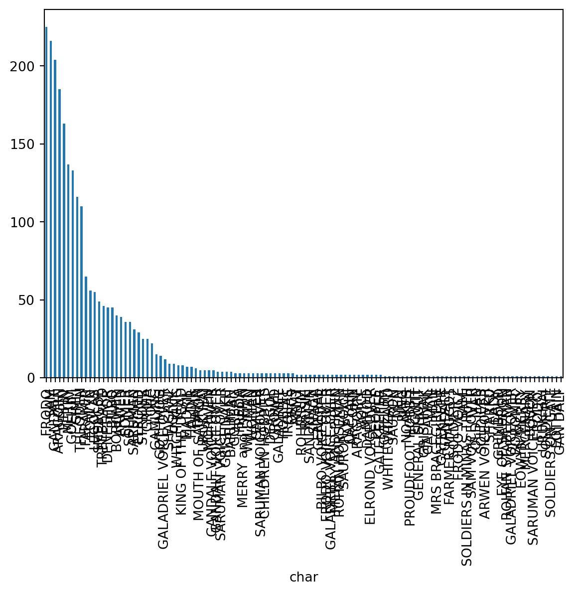

Exercise 2

This plot is messy. We can’t see the names of the characters because they are too long and there are a lot of them. Maybe we could rotate the entire plot so the names are displayed horizontally.

We can do this by using horizontal bar plots. We can create a horizontal bar plot by passing the kind='barh' parameter to the plot() method.

If this doesn’t help, try reducing the number of characters displayed in the plot. You can do this by slicing the result of the value_counts() method.

# create a nicer plot

Filtering data

Sometimes we want to use only a subset of data in our analysis and often we define these subsets based on some condition. For example, we might be interested only in text spoken by Frodo. This is called filtering in a broad sense.

Think of filtering as slicing data, but in this case we are slicing data based on some condition. As in regular slicing, we use square brackets to filter data. The difference is that we pass a condition inside the square brackets.

For example, if we want to filter data to show only the text spoken by Frodo, we can do this by passing the condition data['char'] == 'Frodo' inside the square brackets.

data[data['char'] == 'FRODO']

	char	dialog	movie
16	FRODO	Gandalf?	The Return of the King
17	FRODO	Oooohhh!	The Return of the King
20	FRODO	Gimli!	The Return of the King
25	FRODO	No, it isn't. It isn't midday yet. , The days ...	The Return of the King
30	FRODO	What about you?	The Return of the King
...	...	...	...
2323	FRODO	Yes	The Fellowship of the Ring
2327	FRODO	What are they ?	The Fellowship of the Ring
2329	FRODO	Where are you taking us ?	The Fellowship of the Ring
2332	FRODO	I think a servant of the enemy would look fair...	The Fellowship of the Ring
2334	FRODO	We have no choice but to trust him	The Fellowship of the Ring

225 rows × 3 columns

Exercise 3

Let’s perform a frequency analysis of words spoken by different characters, but this time we will focus only on the final movie of the saga, “The Return of the King”.

# create `rotk` dataframe by filtering the data for the 'Return of the King' movie

# repeat the same steps as above for frequency analysis

Grouping data

Data grouping is one of the most powerful and useful features of Pandas. It allows us to group data based on some criteria and then perform operations on these groups. This often used when we want to transform large dataset into a table which have aggregated data or summary statistics.

Grouping data in Panadas has two componets: grouping and aggregation. Grouping is the process of splitting data into groups based on some criteria. Aggregation is the process of applying a function to each group to get a single value for each group.

Think of grouping as squeezing data into a smaller table. This table will have fewer rows and columns than the original table, but it will contain the same information.

Let’s see how it works by breaking down number of dialogue lines in each movie.

We will first group the data by movie, so we will be using data.groupby('movie'). This will return a DataFrameGroupBy object. On its own, this object is not very useful. We need to apply an aggregation function to it to get some useful information.

In this case, we will use the size() method to count the number of dialogue lines in each group. This method will return a data frame with the number of dialogue lines in each movie.

data.groupby('movie').size()

movie
The Fellowship of the Ring      504
The Return of the King          873
The Two Towers                 1010
dtype: int64

As we can see, the Two Towers has the most dialogue lines, followed by the Return of the King and the Fellowship of the Ring.

This is a simple example of grouping data. Most complex examples require us to explicitely state what data are we aggregating/summarizing and which summary function we are using. This is done by using the agg() method.

Here’s the same example, this time using the agg() method.

data.groupby('movie').agg({'dialog': 'count'})

	dialog
movie
The Fellowship of the Ring	503
The Return of the King	873
The Two Towers	1010

agg() method takes a dictionary as an argument. The keys of the dictionary are the columns we want to aggregate, and the values are the functions we want to apply to these columns.

You can read the code above as:

1. data: we want to process the data stored in this data frame
2. groupby('movie'): we want to groupthe data by the movie column
3. agg({'dialogue': 'count'}): we want to count the number of dialogue lines in each group

Notice that in the final part of the code, we are first interpreting the function (what do we want to do with the data) and then the column (which column do we want to summarize).

Exercise 4

Let’s try to visualize the number of dialogue lines in each movie proportionally. We can do this by creating a pie chart.

Pie charts are created by passing the kind='pie' parameter to the plot() method. Try it in the next cell.

You will notice that we are combining several methods here. This is often the case in data processing and analysis. If you are familiar with R, you will notice that this is very similar to the pipe operator %>% in the dplyr or tidyverse packages.

# your code here

Exercise 5

Which movie has the most unique characters?

# your code here

Tying it all together

We went through basic Pandas methods in this notebook. You’ve seen that often different methods get stacked together to solve a particular problem. We are going to do this for a more complex problem in the final exercise.

Take 10 most frequent characters in the dataset and create a bar plot of the number of dialogue lines spoken by each character in each movie.

This is a complex problem that requires you to combine several methods. You will need to:

1. Filter the data to show only the 10 most frequent characters
2. Group the data by character and movie
3. Aggregate the data to count the number of dialogue lines in each group
4. Create a bar plot of the data

First, let’s filter the data to show only the 10 most frequent characters. We can do this by slicing the result of the value_counts() method. First, let’s see again who the most frequent characters are.

data['char'].value_counts()[0:10]

char
FRODO      225
SAM        216
GANDALF    204
ARAGORN    185
PIPPIN     163
MERRY      137
GOLLUM     133
GIMLI      116
THEODEN    110
FARAMIR     65
Name: count, dtype: int64

If we want to select only names of the characters, we can use the index attribute of the result of the value_counts() method. This attribute returns an array of unique values in the column.

Attributes are similar to methods, but they don’t have parentheses at the end. We call them by using the dot operator, just like methods. Think of attributes as properties of an object.

data['char'].value_counts()[0:10].index

Index(['FRODO', 'SAM', 'GANDALF', 'ARAGORN', 'PIPPIN', 'MERRY', 'GOLLUM',
       'GIMLI', 'THEODEN', 'FARAMIR'],
      dtype='object', name='char')

Let’s save this array in a variable called top_characters.

top_characters = data['char'].value_counts()[0:10].index

Now we will need to make a new data frame that contains only the data of the top 10 characters. Again, filtering is similar to slicing, but we pass a condition inside the square brackets.

In this case the condition is data['char'].isin(top_characters). This condition checks if the value in the char column is in the top_characters array. This will return a new data frame that contains only the data of the top 10 characters.

top_data = data[data['char'].isin(top_characters)]

Let’s see if this did the trick. We can use the value_counts() method to check if the data frame contains only the top 10 characters.

top_data['char'].value_counts()

char
FRODO      225
SAM        216
GANDALF    204
ARAGORN    185
PIPPIN     163
MERRY      137
GOLLUM     133
GIMLI      116
THEODEN    110
FARAMIR     65
Name: count, dtype: int64

Great! Now we can group the data by character and movie and aggregate the data to count the number of dialogue lines in each group. We can do this by using the agg() method.

In this case, we need to group by two columns: char and movie. We can do this by passing a list of columns to the groupby() method: [char', 'movie'].

Why are we grouping by two columns? Because we want to count the number of dialogue lines spoken by each character in each movie. This means that we need to group the data in that order.

top_data.groupby(['char','movie']).agg({'dialog': 'count'})

		dialog
char	movie
ARAGORN	The Fellowship of the Ring	27
	The Return of the King	61
	The Two Towers	97
FARAMIR	The Return of the King	24
	The Two Towers	41
FRODO	The Fellowship of the Ring	70
	The Return of the King	73
	The Two Towers	82
GANDALF	The Fellowship of the Ring	72
	The Return of the King	93
	The Two Towers	39
GIMLI	The Fellowship of the Ring	23
	The Return of the King	34
	The Two Towers	58
GOLLUM	The Fellowship of the Ring	3
	The Return of the King	52
	The Two Towers	78
MERRY	The Fellowship of the Ring	41
	The Return of the King	41
	The Two Towers	55
PIPPIN	The Fellowship of the Ring	38
	The Return of the King	69
	The Two Towers	56
SAM	The Fellowship of the Ring	38
	The Return of the King	91
	The Two Towers	87
THEODEN	The Return of the King	46
	The Two Towers	64

We see interesting things from this table. For example, King Theoden doesn’t speak in the Fellowship of the Ring, but he has a lot of dialogue lines in the Two Towers and the Return of the King. likewise, Gollum has very few lines in the Fellowship of the Ring, but he is featured prominently in the Two Towers and the Return of the King.

Let’s create a bar plot of the data. We can do this by passing the kind='bar' parameter to the plot() method.

top_data.groupby(['char','movie']).agg({'dialog': 'count'}).plot(kind='bar')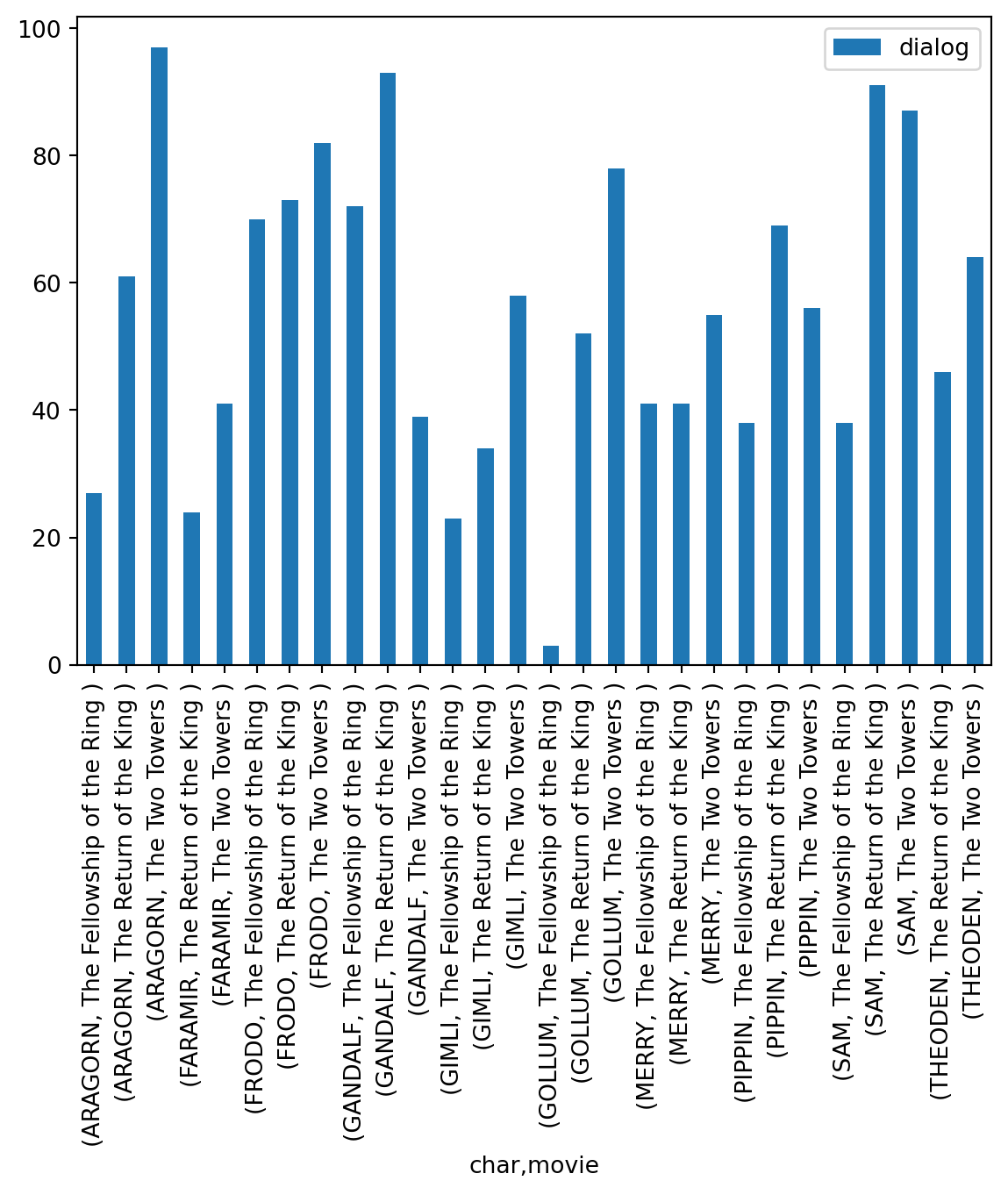

Now, this plot is not good. We have too many labels and it’s not clear which bars represent which movie and character.

We can make this plot better by introducing color legend for the movies. We first achieve this by using the unstack() method. This method will pivot the data frame so that the movies become columns. This will allow us to color the bars by movie (Examine the result of unstack() method to see how the data frame is transformed).

We use unstack() method on the result of the agg() method, right before we call the plot() method.

top_data.groupby(['char','movie']).agg({'dialog': 'count'}).unstack().plot(kind='bar')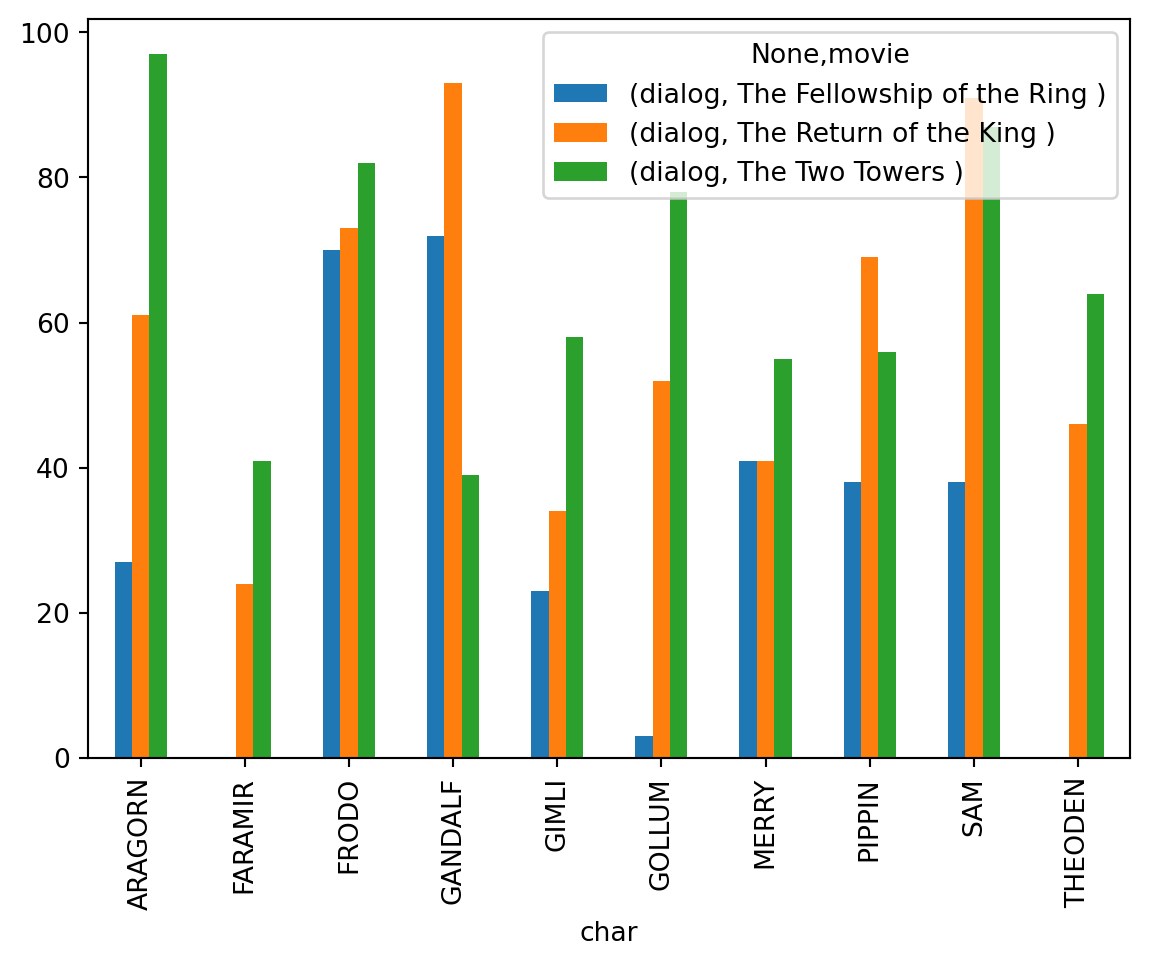

We chained total of 4 methods here: groupby(), agg(), unstack(), and plot() to create this plot.

Exercise 6

It would benefit from further improvements: we can change legend labels, add a title, and rotate the plot so the names of the characters are displayed horizontally.

You can try to solve this issues on your own. Use Pandas documentation, Stack Exchange, chatGPT or any other resource you find useful. Once you know the basics of Python and Pandas, you can solve almost any data processing and analysis problem step by step.

# use unstack and drop one column level so you don't have (dialog, ...) in the legend label

# convert character names to title case

# rename x and y label

# add title to the plot

Conclusion

In this notebook, we learned the basics of Pandas. We learned how to load data, filter data, group data, and visualize data. These are the building blocks of data processing and analysis in Python. You will probably need to combine these methods in different ways when dealing with any task in data analysis or NLP.

We didn’t work with numeric data at all, but once you know the basics of Python and Pandas, the only additional knowledge you will need is to get familiar with new types of methods and attributes that are specific to the data you are working with. The basics principles of slicing, filtering, grouping, and visualizing data are almost the same for all types of data.

This is the topic of the next notebook, which is a take-home assignment. You will need to apply the knowledge you’ve gained in this notebook to a new dataset featuring mix of text and numeric data.